This post is about understanding the difference between a mathematical model and the physical system that is being modeled. Confusion between the model and the physical system is especially prevalent in quantum physics and leads to statements such as:
- A particle can be in two places at once
- An object is spread out in space until you measure it
- Sometimes it’s a particle and sometimes it’s a wave
This post consists of three parts. First we’ll discuss a very simple example of a mathematical model vs a physical system: a ball being thrown into the air. Then we’ll go on to a more interesting example: the heat equation.
Finally, we’ll tackle Schroedinger’s equation. Without worrying about how to solve the equation, we will simply discuss the mathematical function (the model) that the equation refers to. Then we’ll try to see how that function relates to a physical system (sometimes called a “particle”). Hopefully this will clarify why mis-statements like the ones above are so common.
A ball thrown into the air
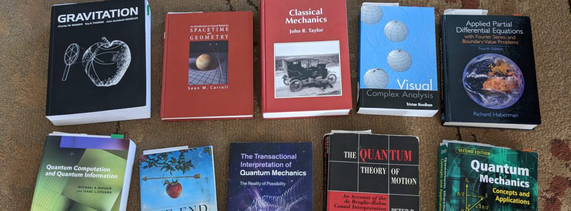
If you throw a ball straight up into the air, its path (ignoring air resistance) can be calculated using Newton’s “2nd law”  . The calculation itself is not important for our purposes, but if we plot the resulting height of the ball for the time it is in the air we get a parabola as in the following diagram:
However, the parabola that appears in the diagram does not appear anywhere in physical space. This sometimes confuses people the first time they see a picture like this. If you don’t notice that the horizontal axis is time it’s easy to imagine that the ball is being thrown from one place to another. In fact, if you do throw a ball from one place to another, its path will be a parabola. But that’s not what we see in the diagram above. That ball is simply going straight up and down in physical space.
This is a very simple example of the difference between a mathematical model (the parabola above) and the physical system it represents (a ball going straight up and down).
The Heat Equation
Another (more interesting) example of the model vs the reality is provided by the heat equation. The simplest form of the heat equation is:
![\[\frac{\partial}{\partial t}T=k\frac{\partial^2}{\partial x^2}T\]](https://physicscafe.org/wp-content/ql-cache/quicklatex.com-2fc42bb0230303d9a7674484ab859d7c_l3.png "Rendered by QuickLaTeX.com")
In this form, the heat equation could represent the temperature inside a narrow tube. The idea is that (in an ideal situation) the tube could be so perfectly insulated that heat only flows out the two ends.
The function 
The function  in the equation above represents the temperature at each point in the tube. When we solve the heat equation, it tells us the value of for any time we choose. We then know the temperature at any point in the tube at that time.
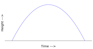
We can imagine the tube lying along the x axis and we could then plot the temperature function , for a given time on the y axis, like so:
Now, even though this is a very common way to visualize the heat equation, if you think about it, it’s kind of a strange mixture of the mathematical model (the blue curve, ) and the physical system that it represents (the gray wire along the x axis). The actual temperature is not a curve hovering above the wire. What the temperature really is, is the motion of the molecules inside the wire.
But there is a straightforward relationship between the blue line and the temperature. Where the line is higher, the molecules are moving faster. So as long as you keep this in mind, it’s easy to keep the two concepts separated and there’s no harm in drawing it all together.
Schroedinger’s Equation
Now we come to Schroedinger’s equation, the fundamental equation used for basic non-relativistic quantum mechanics. This is the equation, in its simplest form:
![\[i\hbar\frac{\partial}{\partial t} \mbox{\Large$\psi$} =-\frac{\hbar^2}{2m} \frac{\partial^2}{\partial x^2} \mbox{\Large$\psi$}\]](https://physicscafe.org/wp-content/ql-cache/quicklatex.com-1e084e5217a905cf97ecc7c82ce51052_l3.png "Rendered by QuickLaTeX.com")
This is the equation that would be used to predict the location of a single particle’s position along the x-axis, if that particle is not being subjected to any forces. We’re not going to solve the equation. We’re simply going to assume that we already have a solution and talk about what that solution means.
The function 
Just as the function was the solution to the heat equation, the function  is the solution to Schroedinger’s equation. But (sometimes called the “wave function” or the “state vector”) is a complex function. That means its values consist of both a real part and an imaginary part. (The imaginary part is a multiple of
  , the square root of
  .)
.)
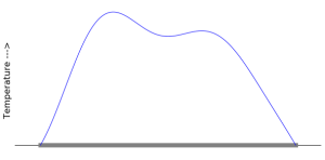
Since is complex, we can’t simply plot its values along the x-axis as we did with . There are various ways that we can attempt to visualize . For example we can plot it in the complex plane. This means we plot the complex values on a real axis vs an imaginary axis, like so:
If we do it this way, then the wave function of this particular particle looks sort of like a spiral.
Another common way to visualize a complex function is to draw the real and imaginary parts separately, as if they were both real, but plot them in different colors. If we take the same wave function above, and plot the real part in blue and the imaginary part in red (both on the real plane) then we get this picture:
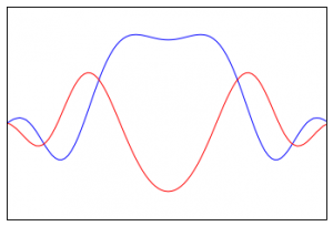
If we do it this way, it looks kind of like two overlapping “waves.”
So what is really? Is it a spiral, is it waves, or what? The answer of course is that it is neither of these things. The wave function exists in an abstract mathematical space. We can try to picture it in various ways, but it is not really any of those pictures.
The relationship between and the position of the particle
Now let’s talk about the relationship between the mathematical function and the physical system. In our first two examples, the ball and the heat equation, we understood from the beginning what the physical system “really was.” We can see the ball going up and down, and we can see how the height of the real ball corresponds to the height of the parabola at a particular time.
With the heat equation, although we can’t actually see the molecules moving around, we can easily form a picture in our minds of what heat consists of in the tube, and we can understand the relationship between the height of the function in the diagram, and how fast those molecules are moving around in the tube lying along the x-axis.
But the relationship between the wave function and our idea of “where a particle is” along the x-axis is much more complicated.
First of all, we don’t use directly, but rather we first apply an operation called the modulus squared. This yields another function  which is actually the probability density function associated with finding the particle at a particular place on the axis.
can be drawn over the x-axis just like we drew the heat function . Here’s a picture of for the same particle above:
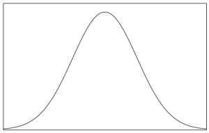
The relationship between the probability density function and the position of the particle is that the area under the curve between two positions on the x-axis gives the probability of finding the particle between those two positions.
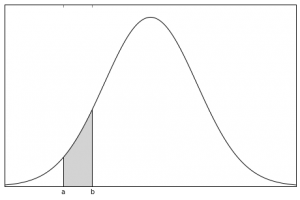
So let’s break that down:
- We are about to look for the particle.
- We want to know the odds that we’ll find it between point a and point b.
- We can find that probability by calculating the area under the curve between those two points.
In case you’re curious, this calculation is done with the integral:
![\[\int_a^b |\psi|^2 dx\]](https://physicscafe.org/wp-content/ql-cache/quicklatex.com-d3da62525f0e19b963907b628ba6fd9d_l3.png "Rendered by QuickLaTeX.com")
We don’t have a “picture” of the particle!
As you can see, the relationship between a particle’s wave function and its position is very different, and much more complicated, than the relationship between the mathematical model and the physical system in our other examples. But the main reason for the confusion between the model and the reality doesn’t (mostly) arise from that fact.
The main issue is that in quantum physics we simply don’t have a “picture” of the particle’s position. When we actually do a measurement, and we see something — say a detector going off — then we typically say that we “saw a particle at position so-and-so.” But, in general, all quantum mechanics gives us is a recipe for calculating the probabilities of these outcomes. It doesn’t say anything about “positions” beyond that.
In fact, there is no universal agreement as to whether there is actually such a thing as a “particle” at the most fundamental level. Some take the position that there are only “quantum fields” and that what we call “particles” are simply excitations in those fields, which can be detected in certain ways under certain circumstances.
So what leads people to say things like the three statements at the beginning of this article? I can only speculate of course, but here are my thoughts.
First of all, they may just be repeating something that they heard or read. This is probably the most likely scenario 🙂
Another possibility is that someone who knows about quantum mechanics, and understands Schroedinger’s equation perfectly well, simply gets confused between the model and the reality. Since we basically don’t know what the “reality” is, this is understandable!
The wave function, and especially the probability density function, do kind of look like something that is “spread out in space.” Furthermore, if you’ve got a picture of the wave function in your head, and the you do a measurement, you could be forgiven for simplifying this mentally, to: “It’s a wave somewhere out there, but then when I measure it, it snaps into position as a particle.”
But even so, why is it that people specifically giving lectures on quantum physics — people who are teaching about the subject — lapse into this kind of language?
I think maybe this is what happens. And it most often happens in “popular” physics book and lectures. You come to the point in the lecture where you have to say something. The “something” that is really true is a purely abstract mathematical statement. But you’re pretty sure your audience won’t understand that, and doesn’t want to hear it. So you fall back on the only “picture” you have, which is a picture of a wave (or probability density) function and you just talk about it as if it were the physical reality.
You probably figure that it will at least give people some kind of notion of what’s going on. Or, at least it will convey a feeling for how unintuitive quantum physics can be. Or, at least it will sound cool …
However, in my view at least, it actually conveys a mistaken impression of “what quantum physics says.”
Final Note
OK, so I get where “spread out in space” and “sometimes a wave” come from. But I still don’t see anything that looks like a particle in “two places at once.”
Right. So the wave function above was for a very simple situation. Basically what’s called a “free particle.” In a more complicated scenario (but still for a single particle) you can ultimately end up with a probability density function that looks something like this:
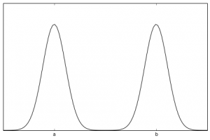
As you can see, there is a pretty strong probability that an experiment will detect the particle either around point a or around point b. The probability is actually non-zero all along the line, but it’s strongly peaked near those two locations. This is where the “two places at once” notion comes from.
I liked what I have read. It makes sense and sounds plausible. Yet, for the completeness sake, I must add that it is only one of possible interpretations. Yes, it allows to predict and verify the prediction, but the Schroedinger’s equation says very little, if anything at all, about the underlying reality. It describes probability distribution for each possible measurements of the system and its evolution over the time. But, again, it does not tell us anything about the causes of this behavior of the nature. We see, we measure, we predict, and that is great. In this sense we “know”. But is it a particle or a wave (as we borrow the images from our immediate experience)? Such a question, I think, does not make sense.
And that is exactly the aspect I like in Mike’s presentation – how he shows the possible reasons for the language we use while describing the phenomenon.
But do not despair. In my experience, after you use this equation for some time and it brings the expected results, you start acquiring a new intuition in the world of quantum. You get used to it and then accept it as the fact of the reality. No more weird than this cup of coffee and the effect of its drinking in the morning.
Well, unless you start asking the question, Why I feel good drinking it? What “why” means? What “feel” means? And what is “good”? I even do not mention that “I” is one of the biggest problems in science today.
Interesting article and comment!
Our basic human senses are typically able to interact with and measure macroscopic objects. But when we start thinking and coming up with ways of observing something that is in the microscopic, nanoscopic, subatomic levels, we see that things in those scales behave differently. And it seems to be weird and people that are not prepared try to still compare the small things with the usual large things to which we are used to interact with in every day life. The thing is that we have to accept that real world is richer than what we normally observe (for example the range of photon wavelengths is effectively infinite, but our eyes can only see a very narrow band of this range). I think it is better to stop arguing about if something is a particle or a wave. We should just think of “objects” with a particular “set of characteristics”. For example a soccer ball has a mass and a momentum when it is moving, angular momentum when it is spinning. An electron has a “rest mass”, charge, angular momentum, spin. A photon has no “rest mass”, but has a momentum. We just need to accept that there are “things” with various unique sets of characteristics. It just so happened that our very limited human senses typically “observe” something that is of comparable size to human’s body and normally has the same set of “usual characteristics”, such as the set that the soccer ball possess.
Every object can be described with a probability density function. It just so happens that objects that have dimensions comparable to human sizes have probability density functions that are mathematically “delta functions” and where the “peak” of the delta function is found to be we call “position of the object”. But for objects in small scales, the probability density function does not have to be necessarily a delta function. We just need to accept that a lot more is possible in the world and instead just think about how to utilize different phenomena from all scales to our human needs and desires.
Maybe it could be easier to understand things if we could forget that we are humans and forget “the usual” and instead imagine that we are just an intelligent consciousness that is exploring the world at all levels. The ultimate goal is to have a very “general” and perhaps “unifying” description of the world’s phenomena.
I agree.